| MAGNABEND HANDYMAN MODEL |
Waveforms in the Magnet
Coil and Flux in the
Magnetic Circuit
This page takes a detailed look at the waveforms that occur in the Handyman Magnabend circuit.
The information is relevant to designers and to anyone interested in electromagnets, but is not needed to manufacture the circuit or the electrical assembly.
(For detailed electrical circuit construction information please go to the following page:
The test circuit for the waveforms on this page:
The oscilloscope Chanels are indicated thus: CH1 in the diagram above.
CH2 is connected to a separate circuit - a Flux Integrator. The integrator is explained in more detail towards the bottom of this page.
Three resistors have been added to the Handyman circuit to facilitate oscilloscope measurements. Two of the resistors form a 100:1 voltage divider across the magnet coil and the third, a 0.1 ohm resistor, facilitates current measurement.
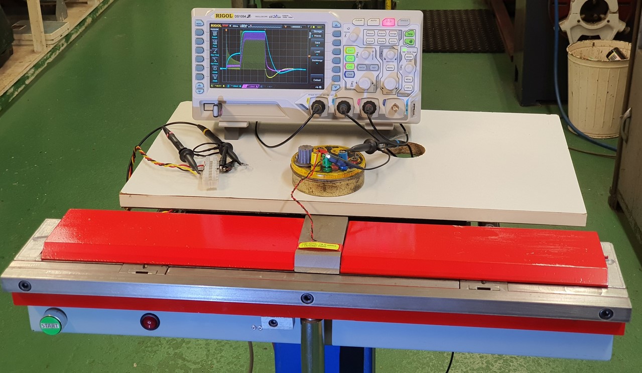
The picture below shows the general setup for measuring the waveforms:
The yellow tobacco tin contains the flux integrator. It is connected to a pickup coil wound on a short (50mm long) piece of clampbar which is placed in the centre of the Handyman magnet top surface. Auxiliary clampbars are placed either side of the sensing clampbar so that flux measurements in the sensing clampbar will be representative of the flux in the whole machine.The oscilloscope probes on the left are connected to the voltage divider and the current monitoring resistor which in turn are connected back into the main circuit as indicated in the diagram above.
The waveforms displayed on the oscilloscope are the result of storing a single sweep during which the switches on the Handyman machine are operated in sequence as required.
_______________________________________________________________
CAUTION !All waveforms shown here were obtained with a Rigol 4-channel digital oscilloscope model DS1054Z. It is important to note that the oscilloscope had to have its earth connection floated for these measurements because the reference for the waveforms is the negative side of the magnet coil and that reference is NOT mains earth.
A safer way to achieve these measurements would have been to use differential oscilloscope probes or optically isolated probes. However such probes are very expensive.
If a battery powered oscilloscope is used then there is no mains earth connection to float, but the following caution will still apply.!
It is most important that the test circuit is powered from an earth leakage protected power outlet (RCD circuit) otherwise you could receive an electric shock if you touch both mains earth and the reference point (or even another point) in the above circuit. (In this circumstance an RCD will provide protection). Even the shell of the probe BNC connectors will be live, although these shells are always insulated on modern oscilloscope probes.
If you wish to perform these tests you should have the appropriate training and experience and you should not touch any bare metal surfaces while mains power is applied to the circuit.
_______________________________________________________________
The oscilloscope traces in the pictures below plot magnet parameters against time and show what happens in the magnet during a bending cycle:-
The magnet coil voltage is represented by the yellow traces,
The magnet coil current is represented by the pink traces and
The magnetic flux in the steel is represented by the blue traces.
Magnabend Waveforms
- Figure
1
Figure 1 shows an overall picture of
a complete bending cycle from light clamping,
through full clamping and the
demagnetising phase which follows the turn-off of power to
the coil.All 3 traces were captured simultaneously and recorded over a time period of 2.4 seconds (the width of the screen).
Magnabend Waveforms
- Figure
2
Figure 2 is an expansion of the first
part of the cycle where only light clamping is applied to the magnet.During this phase the current is limited by the light clamping capacitor (C2 in the circuit diagram). The current builds up to about 0.5 amps during this phase.
(Current was detected by measuring the voltage across a 0.1 ohm resistor in series with the magnet coil.
The oscilloscope sensitivity for the current was set at 120mv/div which translates as 1.2 amps/div).

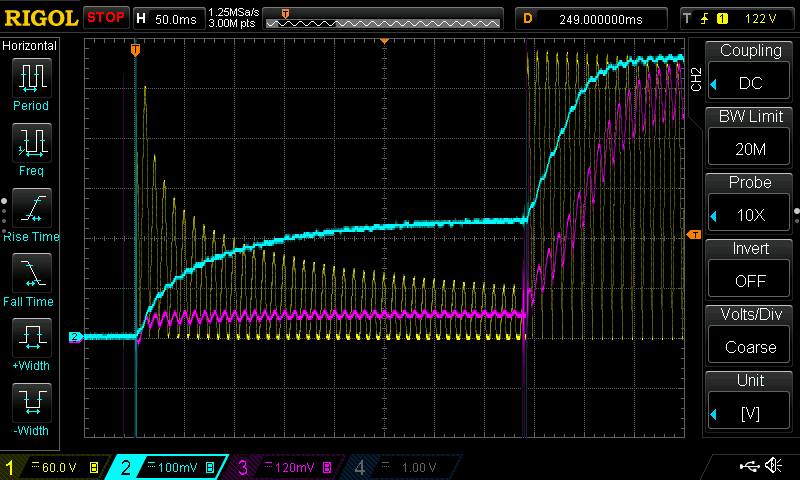
Figure 3
shows the transition from light clamping to full clamping.
The time scale is 20mS/div.
Notice that the voltage (yellow trace) increases instantly but the flux (blue trace) and the current (pink trace) take about 100mS to build up to their maximum values . The flux reaches about 2 Tesla and the current (average of the ripple) reaches about 6 amp.
Notice that the voltage (yellow trace) increases instantly but the flux (blue trace) and the current (pink trace) take about 100mS to build up to their maximum values . The flux reaches about 2 Tesla and the current (average of the ripple) reaches about 6 amp.
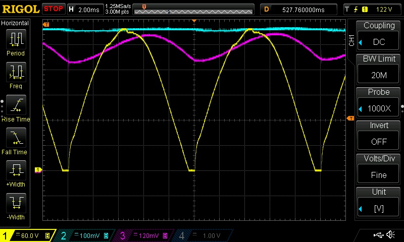
Figure 4 has expanded
the time scale out to 2mS/div and this allows fine detail of the wave
shapes to be observed. Note that the ripple on the current
waveform is phase-shifted by about 35 degrees relative to the voltage
waveform.
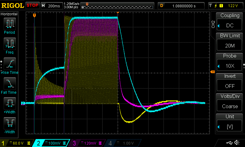
Magnabend Waveforms - Figure 5
Figure 5
shows detail
of the waveforms following the turn-off of AC power
to the circuit. After this the AC part of the circuit (to the left of
the rectifier in the circuit diagram) becomes inactive and is therefore
omitted from the circuit diagrams below. However, because
there is stored energy in the
magnet in the form of its flywheel current and its magnetic field,
interesting things continue to happen in the DC side of the circuit as
discussed below.
(As an aside it should be noted that circuits containg inductors, such as a Magnabend coil, must never be open-circuited while a current is flowing. It is imperative that the flywheel current is afforded a closed path at all times).
 Removal of power does not
result in the relay dropping out instantly but rather it waits
for
about 20mS. That accounts for the flat section on the voltage
waveform (yellow trace) above.
Removal of power does not
result in the relay dropping out instantly but rather it waits
for
about 20mS. That accounts for the flat section on the voltage
waveform (yellow trace) above.
During this wait time the magnet flywheel current will be circulating around thru the rectifier diodes and the (still closed) relay contact.
The magnet energy is being dissipated, mainly thru heating in the coil, and thus the current decays fairly quickly.
Observing the pink trace above it is seen that the initial value of the current is around 6 amps but it drops to around 2.5 amps by the end of the 20mS relay wait time. Thus the magnet coil has already lost most of its stored energy ( Energy = ½ L i2 ) by the time that the relay starts to switch over.
At this stage the relay begins to drop out (switch over) but there will be a brief period, lasting about 3 mS, where the contact is "on-the-fly", that is the contact has left the NO (normally open) contact and is yet to land on the NC (normally closed) contact. This condition is depicted in the circuit diagram below.
While the contact is on-the-fly the magnet flywheel current assumes the red path thru C1 and D1.
D1 carries the magnet current, via C1, for this brief period but does not conduct at any other time in the entire bending cycle.
Nevertheless D1 is very important; without it the relay contact would arc during switch-over and it would probably get melted by the highly inductive magnet flywheel current.
(As an aside it should be noted that circuits containg inductors, such as a Magnabend coil, must never be open-circuited while a current is flowing. It is imperative that the flywheel current is afforded a closed path at all times).
Removal of power does not
result in the relay dropping out instantly but rather it waits
for
about 20mS. That accounts for the flat section on the voltage
waveform (yellow trace) above.During this wait time the magnet flywheel current will be circulating around thru the rectifier diodes and the (still closed) relay contact.
The magnet energy is being dissipated, mainly thru heating in the coil, and thus the current decays fairly quickly.
Observing the pink trace above it is seen that the initial value of the current is around 6 amps but it drops to around 2.5 amps by the end of the 20mS relay wait time. Thus the magnet coil has already lost most of its stored energy ( Energy = ½ L i2 ) by the time that the relay starts to switch over.
At this stage the relay begins to drop out (switch over) but there will be a brief period, lasting about 3 mS, where the contact is "on-the-fly", that is the contact has left the NO (normally open) contact and is yet to land on the NC (normally closed) contact. This condition is depicted in the circuit diagram below.
While the contact is on-the-fly the magnet flywheel current assumes the red path thru C1 and D1.
D1 carries the magnet current, via C1, for this brief period but does not conduct at any other time in the entire bending cycle.
Nevertheless D1 is very important; without it the relay contact would arc during switch-over and it would probably get melted by the highly inductive magnet flywheel current.
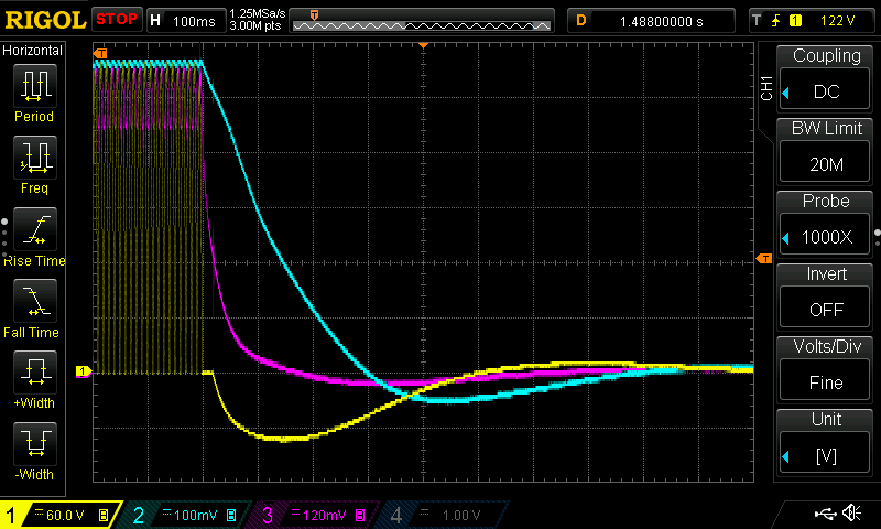
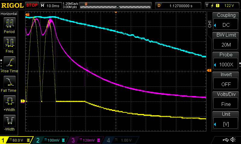
Magnabend Waveforms - Figure 6
Figure 6.
Once the relay has completed its switch-over then the demagnetising phase can begin.
The magnet flywheel current can now circulate thru the capacitor and the NC contact in the relay. Initially the current will flow in a clockwise sense and will be charging the capacitor C1 towards a negative peak (yellow trace above).
Looking at the current waveform in
Figure 6 it can be seen that the current will have fallen to zero after
about
160mS. At this point the capacitor will not receive any more
charge and will begin to discharge back into the magnet coil. The
circulation sense of the current will now be anti-clockwise
around the red loop.
This negative current should induce a reverse flux in the magnet but the effect is delayed because of the inductance of the coil and the eddy currents in the steel.
Eventually however the flux does reverse and reaches a negative peak about 400mS after the relay switch-over.
This negative flux peak is what causes the cancelling of the residual magnetism - demagnetising.
(The transfer of energy between the capacitor and the magnet could, in principal, occur multiple times, i.e. it could oscillate. However in the case of the Magnabend magnet the energy losses in the coil, the so called "I2R" losses, and the losses due to eddy currents in the steel are such that barely one cycle of oscillation occurs, but that is all that is needed for this method of demagnetising to work).
____________________________________________________________
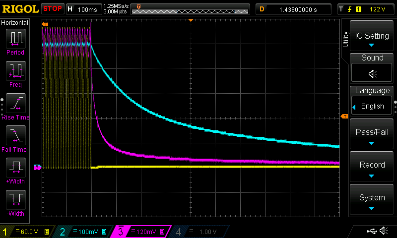
Magnabend Waveforms - Figure 7
Figure 7
shows the waveforms
when the demagnetising capacitor has been removed from the
circuit . As a result there is no negative
pulse on the voltage
waveform, the current does not become negative at all and the flux
decays exponentially but does not get reversed. The net
result is that the clampbars remain weakly clamped to the magnet at the
end of the bending cycle thus making it difficult to remove the
workpiece.
Comparing the waveforms in Figure 6 to those in Figure 7 provides an excellent illustration of the effectiveness of the demagnetising circuit.
Comparing the waveforms in Figure 6 to those in Figure 7 provides an excellent illustration of the effectiveness of the demagnetising circuit.
________________________________________________
In summary it is seen
that the provision of just two simple components, C1 and D1 (in
conjuction with a relay contact) has provided for well controlled
waveforms and a very effective demagnetising circuit.
(By the way other components, on the AC side of the circuit, have nothing to do with demagnetising).
It is thought that other electromagnets, such as magnetic chucks, could benefit from this design.
Note however that this design only works well if C1 is sufficiently large taking into account the magnitude of the magnet current.
The larger the value of C1 then the smaller its voltage rating can be and thus its physical size remains quite moderate.
________________________________________________(By the way other components, on the AC side of the circuit, have nothing to do with demagnetising).
It is thought that other electromagnets, such as magnetic chucks, could benefit from this design.
Note however that this design only works well if C1 is sufficiently large taking into account the magnitude of the magnet current.
The larger the value of C1 then the smaller its voltage rating can be and thus its physical size remains quite moderate.
For the Handyman Magnabend C1 = 1,000µF/63 volts, works well .
For new designs it is suggested to choose C1 = 300µF per amp of coil current.
The
Flux Integrator
The ability to view the magnetic flux provides a powerful insight into what is happening in the Magnabend magnetic circuit.
The flux cannot be seen directly but there are ways of revealing it.
Two electronic means have been used when researching the Magnabend:
- A Hall probe. A Hall probe
generates a voltage
proportional to the magnetic field passing thru it. This type
of probe can be used in conjunction with a voltmeter for
studying steady magnetic fields or it can have an oscilloscope
connected for study of fast changing fields.
- A flux integrator circuit connected to a pickup coil. This method is expanded upon below.
The flux integrator relies on Faraday's
Law of
eletromagnetic induction:- a changing flux within a
coil induces
a voltage on the coil proportional to the rate of change of the
magnetic flux.
For a coil with N turns the voltage generated is given by this equation:
 Because it is only changing flux that
generates a
voltage then it is fundamental that those changes have to
be added up, that is integrated, in order to get
the
total flux.
Because it is only changing flux that
generates a
voltage then it is fundamental that those changes have to
be added up, that is integrated, in order to get
the
total flux.
The integration can be performed electronically with an operational amplifier in a circuit like the one below:
For a coil with N turns the voltage generated is given by this equation:
The integration can be performed electronically with an operational amplifier in a circuit like the one below:
The output voltage of the operational
amplifier, eout,
represents the integral over time of the input voltage, ein.
Substituting for ein in the integral
equation and simplifying we get this nice simple result:-
(The integral equations have been
included here for
the sake of completeness but all we really need to know is the simple
equation above).
Now, mostly we are more interested in the flux density rather than the total flux. To obtain the flux density it is necessary to divide the total flux by the area thru which it is passing.
 For the pickup coil that was used to obtain the
flux waveforms in the
oscilloscope traces above, the relevant area of contact with the front
pole is: 16mm x 50mm.
For the pickup coil that was used to obtain the
flux waveforms in the
oscilloscope traces above, the relevant area of contact with the front
pole is: 16mm x 50mm.
Converting that to area in square metres gives 0.0008 m2.
We
can rearrange the equation to make the flux the
subject and insert values for R and C:
ØB = (eout x RC)/N
= eout x 1.06uF x 266k x 10-3/100
= eout x 0.00282 Weber
Now, mostly we are more interested in the flux density rather than the total flux. To obtain the flux density it is necessary to divide the total flux by the area thru which it is passing.
For the pickup coil that was used to obtain the
flux waveforms in the
oscilloscope traces above, the relevant area of contact with the front
pole is: 16mm x 50mm.Converting that to area in square metres gives 0.0008 m2.
So B = ØB/A = eout x 0.00282/ 0.0008
= 3.53 x eout and the units
will be
webers/m2
i.e. Teslas.

This equation provides a simple way to calculate the flux density corresponding to any voltage reading at the output of the integrator. The constant in the equation is only applicable to the specific parameters used to derive it.
(If desired it would be possible, and perhaps convenient, to make this constant equal to 1. For instance if the number of turns in the pickup coil (N) was increased from 100 to 353 then there would be a one-to-one correspondence between B and and the integrator output voltage. Alternatively the values of R and C could be adjusted etc).
As
an example we can apply this result to the flux waveforms above.
Looking at
the (blue) scope traces in Figure 1 the maximum
flux reading (during full clamping)
is around 560mV (Flux waveform sensitivity is set
to 100mV/ div).
Thus maximum flux density is:
B
= 3.53 x
0.560 Tesla
= 1.98 Tesla .
= 1.98 Tesla .
This is exactly as expected as it is
close to the saturation
flux
density for steel of around 2 Tesla.
(For the waveform measurements above there is no workpiece or air gap present under the test clampbars and therefore magnetic saturation is expected).
This result suggests that the flux integrator is working properly and that the theory presented here is sound.
(For the waveform measurements above there is no workpiece or air gap present under the test clampbars and therefore magnetic saturation is expected).
This result suggests that the flux integrator is working properly and that the theory presented here is sound.
NOTES:
- The slightest offset voltage in the operational amplifier will get integrated and cause the output signal to drift. It is therefore usually necessary to reset the integrator (eg by shorting out the capacitor) before each measurement. Drift can be minimised by fitting a balancing potentiometer to the op amp. (Refer to "offset null" in the op amp data sheet).
- It is best to power the integrator circuit from batteries. Its reference ("earth") can then be tied to the same reference as other oscilloscope probes that might be measuring, for example, the magnet coil voltage.
- The op amp shown in the above circuit is an LH0042. That
type may now be obsolete, but any general purpose op amp could be used
to make the integrator circuit.
This
page last updated: 6 May 2021